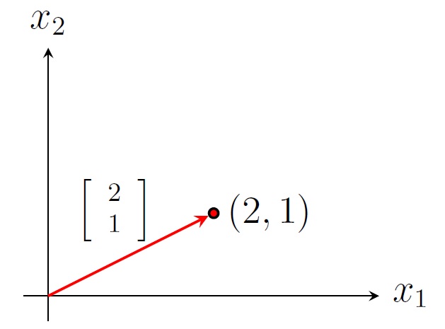
Position vector of a point in the 2-space \(\mathbb R^2\)
Introduction to Linear Algebra |
Matrix: An \(m\times n\) matrix \(A\) is an \(m\)-by-\(n\) array of scalars from a field (for example,
real numbers) of the form
\[A=\left[\begin{array}{cccc}
a_{11}&a_{12}&\cdots &a_{1n}\\
a_{21}&a_{22}&\cdots &a_{2n}\\
\vdots&\vdots&\ddots &\vdots\\
a_{m1}&a_{m2}&\cdots &a_{mn}
\end{array}\right].\]
The order (or size) of \(A\) is \(m\times n\) (read as m by n) if \(A\) has \(m\) rows and
\(n\) columns. The \((i,j)\)-entry of \(A=[a_{i,j}]\) is \(a_{i,j}\).
For example, \(A=\left[\begin{array}{rrr}1&2&0\\-3&0&-1\end{array} \right]\) is a \(2\times 3\) real matrix.
The \((2,3)\)-entry of \(A\) is \(-1\).
Useful matrices:
Position vector of a point in the 2-space \(\mathbb R^2\)
Matrix operations:
Transpose: The transpose of an \(m\times n\) matrix \(A\), denoted by \(A^T\), is an \(n\times m\)
matrix whose columns are corresponding rows of \(A\), i.e., \((A^T)_{ij}=A_{ji}\).
Example.
If \(A=\left[\begin{array}{rrr}1&2&0\\-3&0&-1\end{array} \right]\), then \(A^T=\left[\begin{array}{rr}1&-3\\2&0\\0&-1\end{array} \right]\).
Scalar multiplication: Let \(A\) be a matrix and \(c\) be a scalar. The scalar multiple, denoted
by \(cA\), is the matrix whose entries are \(c\) times the corresponding entries of \(A\).
Example.
If \(A=\left[\begin{array}{rrr}1&2&0\\-3&0&-1\end{array} \right]\), then \(-2A=\left[\begin{array}{rrr}-2&-4&0\\6&0&2\end{array} \right]\).
Sum: If \(A\) and \(B\) are \(m\times n\) matrices, then the sum \(A+B\) is the \(m\times n\) matrix
whose entries are the sum of the corresponding entries of \(A\) and \(B\), i.e., \((A+B)_{ij}=A_{ij}+B_{ij}\).
Example.
If \(A=\left[\begin{array}{rrr}1&2&0\\-3&0&-1\end{array} \right]\) and \(B=\left[\begin{array}{rrr}0&-2&0\\3&0&2\end{array} \right]\),
then \(A+B=\left[\begin{array}{rrr}1&0&0\\0&0&1\end{array} \right]\).
Multiplication:
Matrix-vector multiplication: If \(A\) is an \(m\times n\) matrix and \(\overrightarrow{x}\) is an
\(n\)-dimensional vector, then their product \(A\overrightarrow{x}\) is an \(n\)-dimensional vector whose
\((i,1)\)-entry is \(a_{i1}x_1+a_{i2}x_2+\cdots+a_{im}x_n\), the dot product of the row \(i\) of \(A\) and
\(\overrightarrow{x}\). Note that
\[A\overrightarrow{x}=\left[\begin{array}{c}
a_{11}x_1+a_{12}x_2+\cdots+a_{1n}x_n\\
a_{21}x_1+a_{22}x_2+\cdots+a_{2n}x_n\\
\vdots\\
a_{m1}x_1+a_{m2}x_2+\cdots+a_{mn}x_n\end{array}\right]
=
x_1\left[\begin{array}{c}
a_{11}\\
a_{21}\\
\vdots\\
a_{m1}
\end{array}\right]+
x_2\left[\begin{array}{c}
a_{12}\\
a_{22}\\
\vdots\\
a_{m2}
\end{array}\right]+\cdots+
x_n\left[\begin{array}{c}
a_{1n}\\
a_{2n}\\
\vdots\\
a_{mn}
\end{array}\right].\]
Example.
If \(A=\left[\begin{array}{rrr}1&2&0\\-3&0&-1\end{array} \right]\) and
\(\overrightarrow{x}=\left[\begin{array}{r}1\\-1\\0\end{array} \right]\), then
\(A\overrightarrow{x}=\left[\begin{array}{r}-1\\-3\end{array} \right]\) which is a linear combination
of first and second columns of \(A\) with weights \(1\) and \(-1\) respectively.
Matrix-matrix multiplication: If \(A\) is an \(m\times n\) matrix and \(B\) is an \(n\times p\) matrix,
then their product \(AB\) is an \(m\times p\) matrix whose \((i,j)\)-entry is the dot product the row \(i\)
of \(A\) and the column \(j\) of \(B\).
\[(AB)_{ij}=a_{i1}b_{1j}+a_{i2}b_{2j}+\cdots+a_{im}b_{mj}\]
Example.
For \(A=\left[\begin{array}{rrr}1&2&2\\0&0&2\end{array} \right]\) and \(B=\left[\begin{array}{rr}2&-2\\0&0\\1&1\end{array} \right]\), we have
\(AB=\left[\begin{array}{rr}4&0\\2&2\end{array} \right].\)
Determinant: The determinant of an \(n\times n\) matrix \(A\) is denoted by \(\det A\)
and \(|A|\). It is defined recursively. By hand we will only find determinant of order 2 and
3.
\[\left\vert\begin{array}{rr}a_{11}&a_{12}\\a_{21}&a_{22}\end{array} \right\vert
=a_{11}a_{22}-a_{12}a_{21}.\]
\[\left\vert \begin{array}{rrr}a_{11}&a_{12}&a_{13}\\
a_{21}&a_{22}&a_{23}\\
a_{31}&a_{32}&a_{33}\end{array} \right\vert
=a_{11}\;\begin{vmatrix}a_{22}&a_{23}\\a_{32}&a_{33}\end{vmatrix}
-a_{12}\;\begin{vmatrix}a_{21}&a_{23}\\a_{31}&a_{33}\end{vmatrix}
+a_{13}\;\begin{vmatrix}a_{21}&a_{22}\\a_{31}&a_{32}\end{vmatrix}\;.\]
Example.
\(\left\vert\begin{array}{rrr}
2&1&7\\
-3&0&-8\\
0&1&-3\end{array} \right\vert
=2\;\begin{vmatrix}0&-8\\1&-3\end{vmatrix}
-1\;\begin{vmatrix}-3&-8\\0&-3\end{vmatrix}
+7\;\begin{vmatrix}-3&0\\0&1\end{vmatrix}=-14.\)
Inverse of a matrix: An \(n\times n\) matrix \(A\) is called invertible if there
is an \(n\times n\) matrix \(B\) such that \(AB=BA=I_n.\) Here \(B\) is called the inverse
of \(A\) which is denoted by \(A^{-1}\). So \[AA^{-1}=A^{-1}A=I_n.\]
Example. \(\left[ \begin{array}{rr}a&b\\c&d\end{array} \right]^{-1}=\displaystyle\frac{1}{ad-bc}\left[ \begin{array}{rr}d&-b\\-c&a\end{array} \right]\).
Theorem. An \(n\times n\) matrix \(A\) is invertible iff \(\det A\neq 0\).
\(A^{-1}\) can be found by the Gauss-Jordan row reductions and adjoint formula:
\[A^{-1}=\displaystyle\frac{1}{\det A}\operatorname{adj} A\]
A system of linear equations with \(n\) variables \(x_1,\ldots,x_n\) and \(m\) equations can be written as follows: \[\begin{eqnarray*} \begin{array}{ccccccccc} a_{11}x_1&+&a_{12}x_2&+&\cdots &+&a_{1n}x_n&=&b_1\\ a_{21}x_1&+&a_{22}x_2&+&\cdots &+&a_{2n}x_n&=&b_2\\ \vdots&&\vdots&& &&\vdots&&\vdots\\ a_{m1}x_1&+&a_{m2}x_2&+&\cdots &+&a_{mn}x_n&=&b_m. \end{array} \end{eqnarray*}\] This linear system is equivalent to the matrix equation \(A\overrightarrow{x}=\overrightarrow{b}\), where \[A=\left[\begin{array}{cccc} a_{11}&a_{12}&\cdots &a_{1n}\\ a_{21}&a_{22}&\cdots &a_{2n}\\ \vdots&\vdots& &\vdots\\ a_{m1}&a_{m2}&\cdots &a_{mn} \end{array}\right], \overrightarrow{x}=\left[\begin{array}{c} x_1\\x_2\\ \vdots\\x_n\end{array} \right] \mbox{ and } \overrightarrow{b}=\left[\begin{array}{c} b_1\\b_2\\ \vdots\\b_m \end{array} \right].\] \(A\) is called the coefficient matrix. There are multiple ways to solve the matrix equation \(A\overrightarrow{x}=\overrightarrow{b}\).
Linear independent vectors: \(\overrightarrow{v_1},\overrightarrow{v_2},\ldots,\overrightarrow{v_k}\) are linearly independent if
\[c_1\overrightarrow{v_1}+c_2\overrightarrow{v_2}+\ldots+c_k\overrightarrow{v_k}=\overrightarrow{0}\implies c_1=c_2=\cdots=c_k=0.\]
In other words, \(\overrightarrow{v_1},\overrightarrow{v_2},\ldots,\overrightarrow{v_k}\) are linearly independent if \([\overrightarrow{v_1}\;\overrightarrow{v_2}\;\ldots\;\overrightarrow{v_k}]\overrightarrow{x}=\overrightarrow{0}\) has only the zero solution \(\overrightarrow{x}=\overrightarrow{0}\).
Theorem. Consider \(n\) vectors \(\overrightarrow{v_1},\overrightarrow{v_2},\ldots,\overrightarrow{v_n}\) in
\(\mathbb R^n\). Then the following are equivalent.
Example.
Show that the following vectors are linearly independent: \(\left[\begin{array}{r}2\\-3\\0 \end{array} \right],\;
\left[\begin{array}{r}1\\0\\1 \end{array} \right]
,\; \left[\begin{array}{r}7\\-8\\-3 \end{array} \right]\).
Solution. \(\det\left[\begin{array}{rrr}
2&1&7\\
-3&0&-8\\
0&1&-3\end{array} \right]=-14\neq 0.\) So the vectors are linearly independent. Also note that any 3-dimensional vector can be written as a linear combination of these three vectors.
Span of vectors: The span of \(\overrightarrow{v_1},\overrightarrow{v_2},\ldots,\overrightarrow{v_k}\), denoted by \(\operatorname{Span}\{\overrightarrow{v_1},\overrightarrow{v_2},\ldots,\overrightarrow{v_k}\}\), is the set of all linear combinations of \(\overrightarrow{v_1},\overrightarrow{v_2},\ldots,\overrightarrow{v_k}\).
Example. \(\mathbb R^2=\operatorname{Span}\left\lbrace\left[\begin{array}{r}1\\0 \end{array} \right],\, \left[\begin{array}{r}0\\1 \end{array} \right] \right\rbrace\).
Eigenvalues and eigenvectors: Let \(A\) be an \(n\times n\) matrix. If \(A\overrightarrow{x}=\lambda \overrightarrow{x}\) for some nonzero vector \(\overrightarrow{x}\) and some scalar \(\lambda\), then \(\lambda\) is an eigenvalue of \(A\) and \(\overrightarrow{x}\) is an eigenvector of \(A\) corresponding to \(\lambda\).
Example. Consider \(A=\left[\begin{array}{rr}1&2\\0&3\end{array} \right],\;\lambda=3,\;
\overrightarrow{v}=\left[\begin{array}{r}1\\1\end{array} \right],\;
\overrightarrow{u}=\left[\begin{array}{r}-2\\1\end{array} \right]\).
Since \(A\overrightarrow{v}
=\left[\begin{array}{rr}1&2\\0&3\end{array} \right]\left[\begin{array}{r}1\\1\end{array} \right]
=\left[\begin{array}{r}3\\3\end{array} \right]
=3\left[\begin{array}{r}1\\1\end{array} \right]
=\lambda\overrightarrow{v}\),
\(3\) is an eigenvalue of \(A\) and \(\overrightarrow{v}\) is an eigenvector of \(A\) corresponding to the
eigenvalue \(3\).
Since \(A\overrightarrow{u}
=\left[\begin{array}{rr}1&2\\0&3\end{array} \right]\left[\begin{array}{r}-2\\1\end{array} \right]
=\left[\begin{array}{r}0\\3\end{array} \right]
\neq \lambda\left[\begin{array}{r}-2\\1\end{array} \right]
=\lambda\overrightarrow{u}\)
for all scalars \(\lambda\), \(\overrightarrow{u}\) is not an eigenvector of \(A\).
Note that an eigenvalue can be a complex number and an eigenvector can be a complex vector.
Example. Consider \(A=\left[\begin{array}{rr}0&1\\-1&0\end{array} \right]\).
Since \(\left[\begin{array}{rr}0&1\\-1&0\end{array} \right]\left[\begin{array}{r}1\\i\end{array} \right]
=\left[\begin{array}{r}i\\-1\end{array} \right]
=i\left[\begin{array}{r}1\\i\end{array} \right]\),
\(i\) is an eigenvalue of \(A\) and \(\left[\begin{array}{r}1\\i\end{array} \right]\) is an eigenvector
of \(A\) corresponding to the eigenvalue \(I\).
The characteristic polynomial of \(A\) is \(\det(A-\lambda I)\), a polynomial of \(\lambda\).
The characteristic equation of \(A\) is \(\det(A-\lambda I)=0\).
Since the roots of the characteristic polynomial are the eigenvalues of the \(n\times n\) matrix \(A\), \(A\) has \(n\) eigenvalues, not necessarily distinct. The multiplicity of a root \(\lambda\) in \(\det(A-\lambda I)\)
is the algebraic multiplicity of the eigenvalue \(\lambda\) of \(A\).
Suppose \(\lambda\) is an eigenvalue of the matrix \(A\). Then
\[\operatorname{NS} (A-\lambda I)=\{\overrightarrow{x}\;|\;(A-\lambda I)\overrightarrow{x}=\overrightarrow{O}\}\] is the eigenspace of \(A\) corresponding to the eigenvalue \(\lambda\).
Example. Let \(A=\left[\begin{array}{rr}1&2\\0&3\end{array} \right]\).
Solution. (a) The characteristic polynomial of \(A\) is
\[\det(A-\lambda I)=\left|\begin{array}{cc}1-\lambda& 2\\0&3-\lambda \end{array} \right|=(1-\lambda)(3-\lambda).\]
\(\det(\lambda I-A)=(1-\lambda)(3-\lambda)=0\implies \lambda=1,3\).\\
So \(1\) and \(3\) are eigenvalues of \(A\) with algebraic multiplicities \(1\) and \(1\) respectively.
(b) The eigenspace of \(A\) corresponding to the eigenvalue \(1\) is
\[\operatorname{NS} (A-1I)=\{\overrightarrow{x}\;|\;(A-I)\overrightarrow{x}=\overrightarrow{O}\}.\]
\[(A-1I)\overrightarrow{x}=\overrightarrow{O}\implies\left[\begin{array}{rr}0&2\\0&2\end{array}\right]\left[\begin{array}{r}x_1\\x_2\end{array}\right]=\left[\begin{array}{r}0\\0\end{array}\right]\implies\left\lbrace
\begin{array}{rrl}
&2x_2&=0\\
&2x_2&=0
\end{array}\right.\]
So we get \(x_2=0\) where \(x_1\) is a free variable. Thus
\[\overrightarrow{x}=\left[\begin{array}{r}x_1\\x_2
\end{array}\right]=\left[\begin{array}{c}x_1\\0
\end{array}\right]
=x_1\left[\begin{array}{c}1\\0
\end{array}\right]
\in \operatorname{Span} \left\{\left[\begin{array}{c}1\\0
\end{array}\right]\right\}.\]
Thus the eigenvector of \(A\) corresponding to the eigenvalue \(1\) is
\(\left[\begin{array}{r}1\\0
\end{array}\right]\)
and the eigenspace of \(A\) corresponding to the eigenvalue \(1\) is
\[\operatorname{NS} (A-1I)=\operatorname{Span} \left\{\left[\begin{array}{r}1\\0
\end{array}\right]\right\}.\]
The eigenspace of \(A\) corresponding to the eigenvalue \(3\) is
\[\operatorname{NS} (A-3I)=\{\overrightarrow{x}\;|\;(A-3I)\overrightarrow{x}=\overrightarrow{O}\}.\]
\[(A-3I)\overrightarrow{x}=\overrightarrow{O}\implies\left[\begin{array}{rr}-2&2\\0&0\end{array}\right]\left[\begin{array}{r}x_1\\x_2\end{array}\right]=\left[\begin{array}{r}0\\0\end{array}\right]\implies\left\lbrace
\begin{array}{rrl}
-2x_1&+2x_2&=0
\end{array}\right.\]
So we get \(x_1=x_2\) where \(x_2\) is a free variable. Thus
\[\overrightarrow{x}=\left[\begin{array}{r}x_1\\x_2
\end{array}\right]=\left[\begin{array}{r}x_2\\x_2
\end{array}\right]
=x_2\left[\begin{array}{c}1\\1
\end{array}\right]
\in \operatorname{Span} \left\{\left[\begin{array}{c}1\\1
\end{array}\right]\right\}.\]
Thus the eigenvector of \(A\) corresponding to the eigenvalue \(3\) is \(\left[\begin{array}{r}1\\1
\end{array}\right]\)
and the eigenspace of \(A\) corresponding to the eigenvalue \(3\) is
\[\operatorname{NS} (A-3I)=\operatorname{Span} \left\{\left[\begin{array}{r}1\\1
\end{array}\right]\right\}.\]
Matrix of functions: Entries of an \(m\times n\) matrix \(A\) may be functions of \(x\):
\[A(x)=\left[\begin{array}{cccc}
a_{11}(x)&a_{12}(x)&\cdots &a_{1n}(x)\\
a_{21}(x)&a_{22}(x)&\cdots &a_{2n}(x)\\
\vdots&\vdots& &\vdots\\
a_{m1}(x)&a_{m2}(x)&\cdots &a_{mn}(x)
\end{array}\right].\]
Calculus on matrix of functions: We take limit, derivative, and integration of a matrix \(A(x)\) entry-wise:
\[\begin{align*}
\lim_{x\to a}A(x)&=\left[\begin{array}{cccc}
\displaystyle\lim_{x\to a}a_{11}(x)&\displaystyle\lim_{x\to a}a_{12}(x)&\cdots &\displaystyle\lim_{x\to a}a_{1n}(x)\\
\displaystyle\lim_{x\to a}a_{21}(x)&\displaystyle\lim_{x\to a}a_{22}(x)&\cdots &\displaystyle\lim_{x\to a}a_{2n}(x)\\
\vdots&\vdots& &\vdots\\
\displaystyle\lim_{x\to a}a_{m1}(x)&\displaystyle\lim_{x\to a}a_{m2}(x)&\cdots &\displaystyle\lim_{x\to a}a_{mn}(x)
\end{array}\right],\\
A'(x)&=\left[\begin{array}{cccc}
a_{11}'(x)&a_{12}'(x)&\cdots &a_{1n}'(x)\\
a_{21}'(x)&a_{22}'(x)&\cdots &a_{2n}'(x)\\
\vdots&\vdots& &\vdots\\
a_{m1}'(x)&a_{m2}'(x)&\cdots &a_{mn}'(x)
\end{array}\right],\\
\text{and }\int A(x)\, dx&=\left[\begin{array}{cccc}
\int a_{11}(x)\, dx &\int a_{12}(x)\, dx &\cdots &\int a_{1n}(x)\, dx\\
\int a_{21}(x)\, dx &\int a_{22}(x)\, dx&\cdots &\int a_{2n}(x)\, dx\\
\vdots&\vdots& &\vdots\\
\int a_{m1}(x)\, dx &\int a_{m2}(x)\, dx &\cdots &\int a_{mn}(x)\, dx
\end{array}\right].
\end{align*}\]
Example.
Consider \(A(x)=\left[\begin{array}{cc}e^x&\cos x\\\sin x&2e^{2x}\end{array} \right]\).
Then \(\displaystyle\lim_{x\to 0}A(x)=\left[\begin{array}{cc}1&1\\0&2\end{array} \right]\),
\(A'(x)=\left[\begin{array}{cc}e^x&-\sin x\\ \cos x& 4e^{2x}\end{array} \right]\),
and
\(\int A(x)\, dx=\left[\begin{array}{cc}e^x&\sin x\\-\cos x&e^{2x}\end{array} \right].\)
Last edited