Definition. A function \(T: V \to W\) from a vector space \(V\) to a vector space \(W\) (over the same field) is called a linear transformation if

1. \(T(\overrightarrow{u}+\overrightarrow{v})= T(\overrightarrow{u})+T(\overrightarrow{v})\) for all \(\overrightarrow{u}, \overrightarrow{v} \in V\) and


2. \(T(c\overrightarrow{v})=cT(\overrightarrow{v})\) for for all \(\overrightarrow{v}\in V\) and all scalars \(c\).

In short, a function \(T: V \to W\) is a linear transformation if it preserves the linearity among vectors:
\(T(c\overrightarrow{u}+d\overrightarrow{v})= cT(\overrightarrow{u})+dT(\overrightarrow{v})\) for all \(\overrightarrow{u}, \overrightarrow{v} \in V\) and all scalars \(c,d\).

Definition. The set of all linear transformations from a vector space \(V\) to a vector space \(W\) (over the same field) is denoted by \(L(V,W)\).

Example.

1. For an \(m\times n\) matrix \(A\), \(T:\mathbb R^n\to \mathbb R^m\) defined by \(T(\overrightarrow{x})=A\overrightarrow{x}\) is a linear transformation.


2. \(T:P_n\to P_{n-1}\) defined by \(T(a_0+a_1t+a_2t^2+\cdots+a_{n}t^n)=a_1+2a_2t+\cdots+na_nt^{n-1}\) is a linear transformation.


3. The trace function \(T:M_{n}(\mathbb R) \to \mathbb R\) defined by \(T(A)=\operatorname{tr}(A)\) is a linear transformation.


4. The right shift operator \(T:\mathbb R^{\infty}\to \mathbb R^{\infty}\) defined by \(T(a_1,a_2,a_3,\ldots)=(0,a_1,a_2,a_3,\ldots)\) is a linear transformation.

From the definition of a linear transformation we have the following properties.

Proposition. For a linear transformation \(T: V \to W\),

1. \(T(\overrightarrow{0_V})=\overrightarrow{0_W}\) and


2. for all \(\overrightarrow{v_1}, \ldots,\overrightarrow{v_k} \in V\) and all scalars \(c_1,\ldots,c_k\), \[T(c_1\overrightarrow{v_1}+c_2\overrightarrow{v_2}+\cdots+c_k\overrightarrow{v_k}) = c_1 T(\overrightarrow{v_1})+c_2 T(\overrightarrow{v_2})+\cdots+c_k T(\overrightarrow{v_k}).\]

Example. Consider the function \(T:\mathbb R^3 \to \mathbb R^3\) defined by \(T(x_1,x_2,x_3)=(x_1,x_2,5)\). Since \(T(0,0,0)=(0,0,5) \neq (0,0,0)\), \(T\) is not a linear transformation.

For any given linear transformation \(T: V \to W\), the domain space is \(V\) and the codomain space is \(W\). We study a subspace of the domain space called Kernel or Null Space and a subspace of the codomain space called Image Space or Range.

Definition. The kernel or null space of a linear transformation \(T: V \to W\), denoted by \(\ker (T)\) or \(\ker T\), is the following subspace of \(V\): \[\ker T= \{\overrightarrow{x} \in V \;|\; T(\overrightarrow{x})=\overrightarrow{0_W}\}.\] The nullity of \(T\), denoted by \(\operatorname{nullity}(T)\), is the dimension of \(\ker T\), i.e., \[\operatorname{nullity}(T)=\operatorname{dim}(\ker T).\]
Example. For the linear transformation \(T:M_{n}(\mathbb R) \to M_{n}(\mathbb R)\) defined by \(T(A)=A-A^T\), \[\ker T=\{A\in M_{n}(\mathbb R) \;|\; T(A)=A-A^T=O\}=\{A\in M_{n}(\mathbb R) \;|\; A^T=A\},\] the set of all \(n\times n\) real symmetric matrices. Then \(\operatorname{nullity}(T)=\operatorname{dim}(\ker T)=n(n+1)/2.\)

Definition. The image space or range of a linear transformation \(T: V \to W\), denoted by \(\operatorname{im} (T)\) or \(\operatorname{im} T\) or \(T(V)\), is the following subspace of \(W\): \[\operatorname{im} T= \{T(\overrightarrow{x}) \;|\; \overrightarrow{x} \in V\}.\] The rank of \(T\), denoted by \(\operatorname{rank}(T)\), is the dimension of \(\operatorname{im} T\), i.e., \[\operatorname{rank}(T)=\operatorname{dim}(\operatorname{im} T).\]
Example. For the linear transformation \(T:M_{n}(\mathbb R) \to M_{n}(\mathbb R)\) defined by \(T(A)=A-A^T\), \[\operatorname{im} T=\{A-A^T \;|\; A\in M_{n}(\mathbb R) \},\] the set of all \(n\times n\) real skew-symmetric matrices. Then \[\operatorname{rank}(T)=\operatorname{dim}(\operatorname{im} T)=n(n-1)/2.\]

Theorem.(Rank-Nullity Theorem) Let \(T: V \to W\) be a linear transformation. If \(V\) has finite dimension, then \[\operatorname{rank}(T)+\operatorname{nullity}(T)=\operatorname{dim}(V).\]

Example. For the linear transformation \(T:M_{n}(\mathbb R) \to M_{n}(\mathbb R)\) defined by \(T(A)=A-A^T\), \[\operatorname{rank}(T)+\operatorname{nullity}(T)=\frac{n(n+1)}{2}+\frac{n(n-1)}{2}=n^2 =\operatorname{dim}(M_{n}(\mathbb R) ).\]

Now we discuss two important types of linear transformation.

Definition. Let \(T: V \to W\) be a linear transformation. \(T\) is onto if each \(\overrightarrow{b}\in W\) has a pre-image \(\overrightarrow{x}\) in \(V\) under \(T\), i.e., \(T(\overrightarrow{x})=\overrightarrow{b}\). \(T\) is one-to-one if each \(\overrightarrow{b}\in \mathbb R^m\) has at most one pre-image in \(V\) under \(T\).

Example.

1. The linear transformation \(T:\mathbb R^3 \to \mathbb R^2\) defined by \(T(x_1,x_2,x_3)=(x_1,x_2)\) is onto because each \((x_1,x_2)\in \mathbb R^2\) has a pre-image \((x_1,x_2,0)\in \mathbb R^3\) under \(T\). But \(T\) is not one-to-one because \(T(0,0,0)=T(0,0,1)=(0,0)\), i.e., \((0,0)\) has two distinct pre-images \((0,0,0)\) and \((0,0,1)\) under \(T\).


2. The linear transformation \(T:\mathbb R^2 \to \mathbb R^3\) defined by \(T(x_1,x_2)=(x_1,x_2,0)\) is one-to-one because \(T(x_1,x_2)=T(y_1,y_2) \implies (x_1,x_2,0)=(x_1,x_2,0) \implies (x_1,x_2)=(y_1,y_2)\). But \(T\) is not onto because \((0,0,1)\in \mathbb R^3\) has no pre-image \((x_1,x_2)\in \mathbb R^2\) under \(T\).


3. The linear transformation \(T:\mathbb R^2 \to \mathbb R^2\) defined by \(T(x_1,x_2)=(x_1+x_2,x_1-x_2)\) is one-to-one and onto (exercise).

Theorem. Let \(T: V \to W\) be a linear transformation. Then the following are equivalent.

1. \(T\) is one-to-one.


2. \(\ker T=\{\overrightarrow{0_V}\}\).


3. \(\operatorname{nullity}(T)=0\).

Example. The linear transformation \(T:\mathbb R^2 \to \mathbb R^3\) defined by \(T(x_1,x_2)=(x_1,x_2,0)\) has the standard matrix \(A=[T(\overrightarrow{e_1})\: T(\overrightarrow{e_2}) ] =\left[\begin{array}{rr} 1&0\\ 0&1\\ 0&0 \end{array} \right]\). Note that the columns of \(A\) are linearly independent , \(\ker T=\operatorname{NS}(A)=\{\overrightarrow{0_2}\}\), and \(\operatorname{nullity}(T)=\operatorname{nullity}(A)=0\). Thus \(T\) (i.e., \(\overrightarrow{x} \mapsto A\overrightarrow{x}\)) is one-to-one.

Theorem. Let \(T: V \to W\) be a linear transformation. Then the following are equivalent.

1. \(T\) is onto.


2. \(\operatorname{im} T=W\).


3. \(\operatorname{rank}(T)=\operatorname{dim}(W)\).

Example. The linear transformation \(T:\mathbb R^3 \to \mathbb R^2\) defined by \(T(x_1,x_2,x_3)=(x_1,x_2)\) has the standard matrix \(A=[T(\overrightarrow{e_1})\: T(\overrightarrow{e_3}) \: T(\overrightarrow{e_2})] =\left[\begin{array}{rrr} 1&0&0\\ 0&1&0 \end{array} \right]\). Note that each row of \(A\) has a pivot position, \(\operatorname{im} T=\operatorname{CS}\left(A\right)=\mathbb R^2\), and \(\operatorname{rank}(T)=\operatorname{rank}(A)=2=\dim(\mathbb R^2)\). Thus \(T\) (i.e., \(\overrightarrow{x} \mapsto A\overrightarrow{x}\)) is onto.

Definition. A linear transformation \(T: V \to W\) is an isomorphism if it is one-to-one and onto. When \(T: V \to W\) is an isomorphism, \(V\) and \(W\) are called isomorphic, denoted by \(V\cong W\).

Example.

1. Define \(T:P_{n}\to \mathbb R^{n+1}\) by \(T(a_0+a_1t+\cdots+a_nt^n)=[a_0,a_1,\ldots,a_n]^T\). Verify that \(\ker T=\{\overrightarrow{0}\}\) which implies \(T:P_n\to \mathbb R^{n+1}\) is one-to-one. Also \(T:P_{n}\to \mathbb R^{n+1}\) is onto since each \([a_0\;a_1\;\cdots\;a_n]^T\in \mathbb R^{n+1}\) has a pre-image \(a_0+a_1t+\cdots+a_nt^n \in P_n\) under \(T\). Thus \(T:P_{n}\to \mathbb R^{n+1}\) is an isomorphism and consequently \(P_n\) and \(\mathbb R^{n+1}\) are isomorphic.


2. The left shift operator \(T:\mathbb R^{\infty}\to \mathbb R^{\infty}\) defined by \(T(a_1,a_2,a_3,\ldots)=(a_2,a_3,a_4,\ldots)\) is a linear transformation. Since each \((a_2,a_3,a_4,\ldots) \in R^{\infty}\) has a pre-image \((0,a_2,a_3,\ldots) \in R^{\infty}\) under \(T\), \(T\) is onto equivalently \(\operatorname{im} T=R^{\infty}\). Verify that \[\ker T=\{(a_1,0,0,\ldots) \;|\; a_1\in R \}=\operatorname{Span}\{(1,0,0,\ldots) \}.\] Thus \(T\) is not one-to-one and hence not an isomorphism. Note that ontoness of \(T\) does not imply that \(T\) is one-to-one which may happen when domain and codomain spaces are infinite dimensional.

Theorem. Let \(T: V \to W\) be a linear transformation. If \(V\) and \(W\) have the same finite dimension, then the following are equivalent.

1. \(T\) is an isomorphism.


2. \(T\) is one-to-one.


3. \(\ker T=\{\overrightarrow{0_V}\}\).


4. \(\operatorname{nullity}(T)=0\).


5. \(T\) is onto.


6. \(\operatorname{im} T=W\).


7. \(\operatorname{rank}(T)=\operatorname{dim}(W)\).

Theorem. If \(V\) and \(W\) are isomorphic via an isomorphism \(T:V\to W\), then \(V\) and \(W\) have similar linear algebraic properties such as follows.

1. \(H\) is a subspace of \(V\) if and only if \(T(H)\) is a subspace of \(W\).


2. \(\{\overrightarrow{v_1},\ldots,\overrightarrow{v_n}\}\) is linearly independent in \(V\) if and only if \(\{T(\overrightarrow{v_1}),\ldots,T(\overrightarrow{v_n})\}\) is linearly independent in \(W\).


3. \(\{\overrightarrow{v_1},\ldots,\overrightarrow{v_n}\}\) spans \(V\) if and only if \(\{T(\overrightarrow{v_1}),\ldots,T(\overrightarrow{v_n})\}\) spans \(W\).


4. \(\{\overrightarrow{v_1},\ldots,\overrightarrow{v_n}\}\) is a basis of \(V\) if and only if \(\{T(\overrightarrow{v_1}),\ldots,T(\overrightarrow{v_n})\}\) is a basis of \(W\).


5. \(\operatorname{dim}(V)=\operatorname{dim}(W)\).

Remark. The preceding theorem is true even when \(V\) and \(W\) have infinite dimensions.

Example. Consider the following three polynomials of \(P_2\): \[\overrightarrow{p_1}(t)=1+t^2, \overrightarrow{p_2}(t)=-1+2t-t^2, \mbox{and }\overrightarrow{p_3}(t)=-1+4t.\] Show that \(\{\overrightarrow{p_1},\;\overrightarrow{p_2},\;\overrightarrow{p_3}\}\) is a basis of \(P_2\).

Solution. First recall that \(T:P_{2}\to \mathbb R^3\) defined by \(T(a_0+a_1t+a_2t^2)=[a_0,a_1,a_2]^T\) is an isomorphism. \[\begin{align*} T(\overrightarrow{p_1})&=T(1+t^2)=\left[\begin{array}{r}1\\0\\1\end{array}\right]\\ T(\overrightarrow{p_2})&=T(-1+2t-t^2)=\left[\begin{array}{r}-1\\2\\-1\end{array}\right]\\ T(\overrightarrow{p_3})&=T(-1+4t)=\left[\begin{array}{r}-1\\4\\0\end{array}\right] \end{align*}\] Now \(A=[T(\overrightarrow{p_1})\;T(\overrightarrow{p_2})\;T(\overrightarrow{p_3})] =\left[\begin{array}{rrr}1&-1&-1\\0&2&4\\1&-1&0\end{array}\right]\xrightarrow{-R1+R3} \left[\begin{array}{rrr}\boxed{1}&-1&-1\\0&\boxed{2}&4\\0&0&\boxed{1}\end{array}\right].\) Since \(3\times 3\) matrix \(A\) has 3 pivot positions, by the IMT, the columns of \(A\) are linearly independent and span \(\mathbb R^3\). Thus \(\{T(\overrightarrow{p_1}),T(\overrightarrow{p_2}),T(\overrightarrow{p_3})\}\) is a basis of \(\mathbb R^3\). Since \(T:P_{2}\to \mathbb R^3\) is an isomorphism, \(\{\overrightarrow{p_1},\;\overrightarrow{p_2},\;\overrightarrow{p_3}\}\) is a basis of \(P_2\).

Definition. Suppose \(B=\left(\overrightarrow{b_1},\ldots, \overrightarrow{b_n}\right)\) is an ordered basis of a real vector space \(V\). Then any vector \(\overrightarrow{x}\in V\) can be written as \(\overrightarrow{x}=c_1\overrightarrow{b_1}+c_2\overrightarrow{b_2}+\cdots+c_n\overrightarrow{b_n}\) for some unique scalars \(c_1,c_2,\ldots,c_n\). The coordinate vector of \(\overrightarrow{x}\) relative to \(B\) or the \(B\)-coordinate of \(\overrightarrow{x}\), denoted by \([\overrightarrow{x}]_B\), is \[[x]_B=[c_1b_1+c_2b_2+\cdots+c_nb_n]_B=\left[\begin{array}{c}c_1\\c_2\\ \vdots \\c_n\end{array}\right].\]

Remark. \([\;\;]_B:V\to \mathbb R^n\) is an isomorphism.

Theorem. If \(V\) is a real vector space of dimension \(n\), then \(V\) is isomorphic to \(\mathbb R^n\).

Definition. Let \(V\) and \(W\) be real vector spaces with ordered bases \(B=\left(\overrightarrow{b_1},\ldots, \overrightarrow{b_n}\right)\) and \(C=\left(\overrightarrow{c_1},\ldots, \overrightarrow{c_m}\right)\) respectively. Let \(T:V\to W\) be a linear transformation. 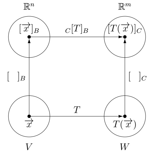The matrix of \(T\) from \(B\) to \(C\), denoted by \([T]_{C\leftarrow B}\) or \(_{C}[T]_B\), is the following \(m\times n\) matrix: \[_{C}[T]_B=\left[ [T(\overrightarrow{b_1})]_C \cdots [T(\overrightarrow{b_n})]_C\right].\] Note that for all \(\overrightarrow{x}\in V\), \[[T(\overrightarrow{x})]_C=_{C}[T]_B [\overrightarrow{x}]_B.\]

The following diagram shows the "equivalence" of a linear transformation \(T:V\to W\) and the corresponding matrix transformation \(_{C}[T]_B: \mathbb R^n\to \mathbb R^m\).

Example. \(P_n\) and \(P_{n-1}\) are real vector spaces with ordered bases \(B=\left(1,x,\ldots,x^n\right)\) and \(C=\left(1,x,\ldots,x^{n-1}\right)\) respectively. For the linear transformation \(T:P_n\to P_{n-1}\) defined by \(T(a_0+a_1x+a_2x^2+\cdots+a_{n}x^n)=a_1+2a_2x+\cdots+na_nx^{n-1}\), we have \[_{C}[T]_B =\left[\begin{array}{ccccc}0&1&0&\cdots&0\\ 0&0&2&\cdots&0\\ \vdots&\vdots&\vdots&\ddots&\vdots\\ 0&0&0&\cdots&n \end{array}\right].\] The columns of \(_{C}[T]_B\) are calculated as follows: \[\begin{align*} \text{Column 1} &:\; [[T(1)]_C=[0]_C=[0\cdot 1+0 x+0x^2+\cdots +0x^{n-1}]_C=[0,0,0\ldots,0]^T\\ \text{Column 2} &:\; [[T(x)]_C=[1]_C=[1\cdot 1+0 x+0x^2+\cdots +0x^{n-1}]_C=[1,0,0,\ldots,0]^T\\ \text{Column 3} &:\; [[T(x^2)]_C=[2x]_C=[0\cdot 1+2 x+0x^2+\cdots +0x^{n-1}]_C=[0,2,0,\ldots,0]^T\\ \vdots &\\ \text{Column n+1} &:\; [[T(x^n)]_C=[nx^{n-1}]_C=[0\cdot 1+0 x+\cdots +0x^{n-2}+nx^{n-1}]_C=[0,0,\ldots,0,n]^T\\ \end{align*}\]

The following theorem shows the relation between two matrices of a linear transformation corresponding to different bases.

Theorem. Let \(V\) be a real vector space with ordered bases \(B\) and \(B'\). Let \(W\) be a real vector space with ordered bases \(C\) and \(C'\). For a linear transformation \(T:V\to W\), \[_{C'}[T]_{B'} =_{C'}[I]_C\; {}_{C}[T]_B\; {}_{B}[I]_{B'} .\]

Last edited