The Euler's method is the simplest way to solve the IVP (1) but it has error \(O(h^2)\). The Taylor's method of order \(k\) has error \(O(h^{k+1})\) which is small, but it involves calculating higher order derivative which is computationally expensive. So in 1901 Carl Runge and Martin Kutta developed a method with high accuracy that does not involve calculating derivatives.

A general form of the second order Runge-Kutta method is the following: \[\begin{array}{lrl} &y_{i+1} &=y_i+h\Big[ c_1k_1+c_2k_2 \Big],\\ \text{where}& &\\ & k_1 &= f(t_i,y_i),\\ & k_2 &= f(t_i+\alpha h,y_i+\beta hk_1). \end{array}\] Different values of \(c_1,c_2,\alpha,\beta\) give different second order Runge-Kutta methods.

By the preceding derivation, we get \[\begin{align*} c_1+c_2 &=1\\ c_2\alpha &=\frac{1}{2}\\ c_2\beta &=\frac{1}{2} \end{align*}\]

There are many solutions for \(c_1,c_2,\alpha,\beta\). One solution is \[(c_1,c_2,\alpha,\beta)=\left(\frac{1}{2},\frac{1}{2},1,1 \right)\] which gives a special second order Runge-Kutta method with error \(O(h^3)\) called the modified Euler's method or "RK2": \[\boxed{\begin{array}{lrl} &y_{i+1} &=y_i+\displaystyle\frac{h}{2}\Big[k_1+k_2 \Big],\\ \text{where}& &\\ & k_1 &= f(t_i,y_i),\\ & k_2 &= f(t_i+h,y_i+hk_1). \end{array}}\] Another solution \((c_1,c_2,\alpha,\beta)=\left(0,1,\frac{1}{2},\frac{1}{2} \right)\) gives another second order Runge-Kutta method called the midpoint method: \[ y_{i+1} =y_i+ hk_2,\; \text{where } k_1= f(t_i,y_i), \; k_2= f\Big(t_i+\frac{h}{2},y_i+\frac{h}{2}k_1 \Big).\]

Example. Use Runge-Kutta method of order 2 with step size \(h=0.5\) to approximate the solution of the following IVP: \[\frac{dy}{dt}=t^2-y,\, 0\leq t\leq 2,\, y(0)=1\] Solution. We have \(h=0.5,\, t_0=0,\, y_0=1\) and \(y'=f(t,y)=t^2-y\). So we have \[\begin{array}{rl} k_1 &= f(t_i,y_i)=t_i^2-y_i,\\ k_2 &= f(t_i+h,y_i+hk_1)\\ &= f(t_i+0.5,y_i+0.5(t_i^2-y_i))\\ &= (t_i+0.5)^2-(y_i+0.5(t_i^2-y_i))\\ &= 0.25(2t_i^2+4t_i+1-2y_i),\\ y_{i+1} &=y_i+\displaystyle\frac{h}{2}\Big[k_1+k_2 \Big]\\ &=y_i+\frac{0.5}{2}\Big[(t_i^2-y_i)+0.25(2t_i^2+4t_i+1-2y_i) \Big] =\frac{6t_i^2+4t_i+1+10y_i}{16}. \end{array}\] \[\begin{align*} t_1&=0+1\cdot 0.5=0.5, &&y_1=(6t_0^2+4t_0+1+10y_0)/16=0.6875\\ t_2&=0+2\cdot 0.5=1, &&y_2=(6t_1^2+4t_1+1+10y_1)/16=0.7109 \; \text{etc.} \end{align*}\] \[\begin{array}{|c|l|l|} \hline i & t_i & y_i \\ \hline 0&0 &1\\ \hline 1&0.5 &0.6875 \\ \hline 2&1 &0.7109\\ \hline 3&1.5 &1.1318\\ \hline 4&2 &1.9886\\ \hline \end{array}\]

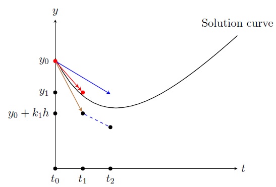
Geometric interpretation: At \((t_0,y_0)\) we draw a line with slope \(k_1=y'(t_0)=f(t_0,y_0)\): \[y=y_0+k_1 (t-t_0).\] At \(t=t_1\), we get the point \((t_1,y_0+k_1h)\) on the line. Now at \((t_1,y_0+k_1h)\) we draw a line with slope \(k_2=f(t_1,y_0+k_1h)\): \[y=(y_0+k_1h)+k_2 (t-t_1).\] Now we go back to the point \((t_0,y_0)\) and draw a line with slope \((k_1+k_2)/2\): \[y=y_0+\frac{k_1+k_2}{2} (t-t_0).\] At \(t=t_1\), the height of the last line is \(y_0+\frac{k_1+k_2}{2}h=:y_1\).

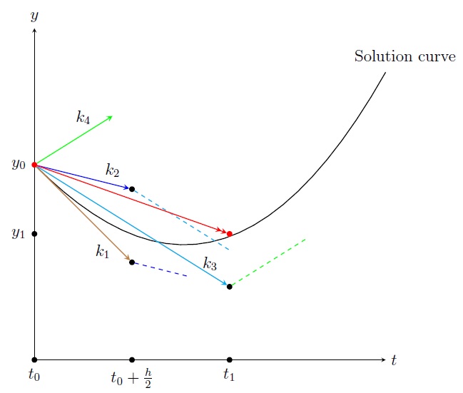
The most widely known Runge-Kutta method is "RK4", the following fourth order Runge-Kutta method with error \(O(h^5)\): \[\boxed{\begin{array}{lrl} &y_{i+1} &=y_i+\displaystyle\frac{h}{6}\Big[ k_1+2k_2+2k_3+k_4 \Big],\\ \text{where}& &\\ & k_1 &= f(t_i,y_i),\\ & k_2 &=\displaystyle f \left(t_i+\frac{h}{2},y_i+k_1\frac{h}{2} \right),\\ & k_3 &=\displaystyle f \left(t_i+\frac{h}{2},y_i+k_2\frac{h}{2} \right),\\ & k_4 &= f(t_i+h,y_i+k_3h). \end{array}}\] So the basic idea is to draw a line at \((t_i,y_i)\) with slope \(m\): \(y=y_i+m (t-t_i)\) where \(m\) is the weighted average of slopes \(k_1,k_2,k_3,k_4\). Then height of the line at \(t=t_{i+1}\), is \(y_i+mh=:y_{i+1}\).

Example. Use Runge-Kutta method of order 4 with step size \(h=0.5\) to approximate the solution of the following IVP: \[\frac{dy}{dt}=t^2-y,\, 0\leq t\leq 2,\, y(0)=1\] Solution. We have \(h=0.5,\, t_0=0,\, y_0=1\) and \(y'=f(t,y)=t^2-y\). So we have \[\begin{array}{rl} k_1 &= f(t_i,y_i)=t_i^2-y_i,\\ k_2 &=\displaystyle f\left(t_i+\frac{h}{2},y_i+k_1\frac{h}{2}\right)= f(t_i+0.25,y_i+0.25k_1)= (t_i+0.25)^2-(y_i+0.25k_1),\\ k_3 &=\displaystyle f\left(t_i+\frac{h}{2},y_i+k_2\frac{h}{2}\right)= f(t_i+0.25,y_i+0.25k_2)= (t_i+0.25)^2-(y_i+0.25k_2),\\ k_4 &= f(t_i+h,y_i+k_3h)= f(t_i+0.5,y_i+0.5k_3)=(t_i+0.5)^2-(y_i+0.5k_3) \\ y_{i+1} &=y_i+\displaystyle\frac{h}{6}\Big[k_1+2k_2+2k_3+k_4 \Big]=y_i+\frac{0.5}{6}\Big[k_1+2k_2+2k_3+k_4 \Big]. \end{array}\] \[\begin{array}{|c|l|l|l|l|l|l|l|} \hline i & t_i & y_i & k_1 & k_2 & k_3 & k_4 & y_{i+1}\\ \hline 0&0 &1 &-1 &-0.6875 &-0.7656 &-0.3671 &0.6438\\ \hline 1&0.5 &0.6438 &-0.3938 &0.0170 &-0.0856 &0.3989 &0.6328\\ \hline 2&1 &0.6328 &0.3671 &0.8378 &0.7201 &0.1257 &1.0278\\ \hline 3&1.5 &1.0278 &1.2221 &1.7290 &1.6023 &2.1709 &1.8658\\ \hline 4&2 &1.8658 &--- &--- &--- &--- &---\\ \hline \end{array}\]

Last edited