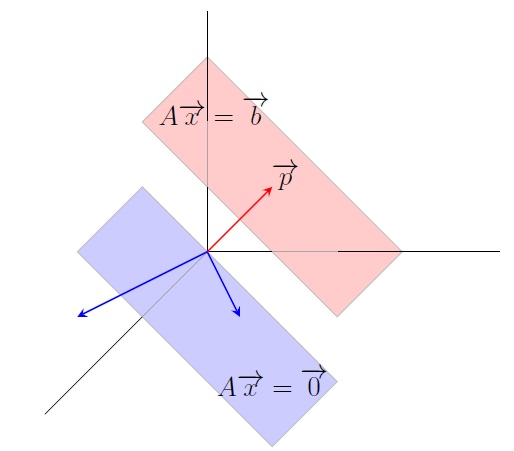
The solution set of \(A\overrightarrow{x}=\overrightarrow{b}\) is a translation of that of \(A\overrightarrow{x}=\overrightarrow{0}\)
Geometry of Solution Sets |
Homogeneous linear system: A system of linear equations is homogeneous if its matrix equation is \(A\overrightarrow{x}=\overrightarrow{0}\). Note that \(\overrightarrow{0}\) is always a solution called the trivial solution. Any nonzero solution is called a nontrivial solution.
Example.
Remark. If \(A\overrightarrow{x}=\overrightarrow{0}\) has \(k\) free variables, then its solution set is the span of \(k\) vectors.
The solution set of \(A\overrightarrow{x}=\overrightarrow{0}\) is
\(\operatorname{Span}\{\overrightarrow{v_1},\ldots,\overrightarrow{v_k}\}\) for some vectors
\(\overrightarrow{v_1},\ldots,\overrightarrow{v_k}\).
The solution set of \(A\overrightarrow{x}=\overrightarrow{b}\) is
\(\{\overrightarrow{p}+\overrightarrow{v}\:|\: A\overrightarrow{v}=\overrightarrow{0}\}\) where
\(A\overrightarrow{p}=\overrightarrow{b}.\)
So a nonhomogenous solution is a sum of a particular solution and a homogeneous solution. To justify it,
let \(\overrightarrow{y}\) be a solution of \(A\overrightarrow{x}=\overrightarrow{b}\), i.e., \(A\overrightarrow{y}=\overrightarrow{b}\).
Then
\[A(\overrightarrow{y}-\overrightarrow{p})=\overrightarrow{b}-\overrightarrow{b}=\overrightarrow{0}.\]
Then \((\overrightarrow{y}-\overrightarrow{p})=\overrightarrow{v}\) where \(A\overrightarrow{v}=\overrightarrow{0}\).
Thus \(\overrightarrow{y}=\overrightarrow{p}+\overrightarrow{v}\).
Geometrically we get the solution set of \(A\overrightarrow{x}=\overrightarrow{b}\) by shifting the solution set
of \(A\overrightarrow{x}=\overrightarrow{0}\) to the point whose position vector is \(\overrightarrow{p}\)
along the vector \(\overrightarrow{p}\).
Example. The nonhomogeneous system \(x_1-x_2-2x_3=-2\) has a particular solution \(\overrightarrow{p}=\left[\begin{array}{r} 1\\ 1\\ 1 \end{array} \right]\). The corresponding homogeneous system \(x_1-x_2-2x_3=0\) has the solution set \[\left\lbrace s \left[\begin{array}{r}1\\ 1\\ 0 \end{array} \right] +t \left[\begin{array}{r}2\\ 0\\ 1 \end{array} \right] \; |\; s,t\in \mathbb R \right\rbrace.\] Thus the solution set of the nonhomogeneous system \(x_1-x_2-2x_3=-2\) is \[\left\lbrace \left[\begin{array}{r} 1\\ 1\\ 1 \end{array} \right] +s \left[\begin{array}{r}1\\ 1\\ 0 \end{array} \right] +t \left[\begin{array}{r}2\\ 0\\ 1 \end{array} \right] \; |\; s,t\in \mathbb R \right\rbrace.\]
The solution set of \(A\overrightarrow{x}=\overrightarrow{b}\) is a translation of that of
\(A\overrightarrow{x}=\overrightarrow{0}\)
Last edited