Euler's Method |
Introduction to IVP: In this chapter we numerically solve the following IVP (initial value problem):
\[\frac{dy}{dt}=f(t,y),\,a\leq t\leq b,\, y(a)=c \;\;\;\;\;\;\;\;\;\;\;\; (1) \]
Instead of finding \(y=y(t)\) on \([a,b]\), we break \([a,b]\) into \(n\) subintervals
\([t_0,t_1],[t_1,t_2],\ldots,[t_{n-1},t_n]\) and approximate \(y(t_i),\,i=0,1,\ldots,n\). But if we need \(y(t)\),
it can be approximated by the Lagrange polynomial \(P_n\) using \(t_0,t_1,\ldots,t_n\).
Before approximating a solution \(y=y(t)\), we must ask if the IVP (1) has a solution and it is unique on \([a,b]\).
The answer is given by the Existence and Uniqueness Theorem:
Theorem. The IVP (1) has a unique solution \(y(t)\) on \([a,b]\) if
When we approximate \(y(t_i),\,i=0,1,\ldots,n\) for the unique solution \(y(t)\), we might commit some round-off errors.
So we ask if the IVP (1) is well-posed:
a small change in the problem (i.e., small change in \(f,c\)) gives a small change in the solution.
It can be proved that the IVP (1) is well-posed if \(f\) satisfies a Lipschitz condition on \(D\). Also note that if
\(|f_y(t,y)|\leq L\) on \(D\), then \(f\) satisfies a Lipschitz condition on \(D\) with constant \(L\).
Euler's Method: We break \([a,b]\) into \(n\) subintervals \([t_0,t_1],[t_1,t_2],\ldots,[t_{n-1},t_n]\) where
\(t_i=a+ih\) and \(h=(b-a)/n\). The Euler's Method finds \(y_0,y_1,\ldots,y_n\) such that
\(y_i\approx y(t_i),\,i=0,1,\ldots,n\):
\[\boxed{
\begin{aligned}
y_0 &=c\\ y_{i+1} &=y_i+hf(t_i,y_i),\, i=0,1,\ldots,n-1.
\end{aligned}}\]
To justify the iterative formula, use Taylor's theorem on \(y\) about \(t=t_i\): \[\begin{array}{rrl} &y(t) &= y(t_i)+(t-t_i)y'(t_i)+\frac{(t-t_i)^2}{2}y''(\xi_i)\\ \implies &y(t_{i+1}) &= y(t_i)+(t_{i+1}-t_i)y'(t_i)+\frac{(t_{i+1}-t_i)^2}{2}y''(\xi_i)\\ & &= y(t_i)+hf(t_i,y(t_i))+\frac{h^2}{2}y''(\xi_i)\\ \implies & y(t_{i+1})& \approx y_i+hf(t_i,y_i) =: y_{i+1} \end{array}\]
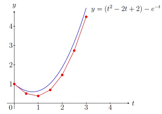
Example. Use Euler's method with step size \(h=0.5\) to approximate the solution of the following IVP: \[\frac{dy}{dt}=t^2-y,\, 0\leq t\leq 3,\, y(0)=1\] Solution. We have \(h=0.5,\, t_0=0,\, y_0=1\) and \(f(t,y)=t^2-y\). So \[y_{i+1}=y_i+0.5(t_i^2-y_i)=0.5(t_i^2+y_i).\] \[\begin{align*} t_1&=0+1\cdot 0.5=0.5, &&y_1=0.5(t_0^2+y_0)=0.5(0+1)=0.5\\ t_2&=0+2\cdot 0.5=1, &&y_2=0.5(t_1^2+y_1)=0.5(0.25+0.5)=0.375 \; \text{etc.} \end{align*}\] \[\begin{array}{|c|l|l|} \hline i & t_i & y_i \\ \hline 0&0 &1\\ \hline 1&0.5&0.5\\ \hline 2&1 &0.375\\ \hline 3&1.5&0.6875\\ \hline 4&2 &1.46875\\ \hline 5&2.5&2.734375\\ \hline 6&3 &4.4921875\\ \hline \end{array}\]
Geometric Interpretation: The tangent line to the solution \(y=y(t)\) at the point \((t_0,y_0)\) has slope \(\displaystyle\left.\frac{dy}{dt}\right]_{(t_0,y_0)}=f(t_0,y_0)\). So an equation of the tangent line is \[y=y_0+(t-t_0)f(t_0,y_0).\] If \(t_1\) is close to \(t_0\), then \(y_1=y_0+(t_1-t_0)f(t_0,y_0)=y_0+hf(t_0,y_0)\) would be a good approximation to \(y(t_1)\). Similarly if \(t_2\) is close to \(t_1\), then \(y(t_2)\approx y_2=y_1+hf(t_1,y_1)\).
Maximum error: Suppose \(D=\{(t,y)\,|\, a\leq t\leq b,\, -\infty< y< \infty \}\) and \(f\) satisfies a Lipschitz condition on \(D\) with constant \(L\). Suppose \(y(t)\) is the unique solution to (1) where \(|y''(t)|\leq M\) for all \(t\in [a,b]\). Then for the approximation \(y_i\) of \(y(t_i)\) by the Euler's method with step size \(h\), we have \[|y(t_i)-y_i|\leq \frac{hM}{2L}\left[ -1+e^{L(t_i-a)} \right],\, i=0,1,\ldots,n.\]
Example.
Find the maximum error in approximating \(y(1)\) by \(y_2\) in the preceding example. Compare it with the actual absolute
error using the solution \(y=(t^2-2t+2)-e^{-t}\).
Solution. \(f(t,y)=t^2-y \implies |f_y|=|-1|\leq 1=L\) for all \(y\). Thus \(f\) satisfies a Lipschitz condition on
\(D=(0,3)\times(-\infty,\infty)\) with the constant \(L=1\). Now
\[y=(t^2-2t+2)-e^{-t} \implies y''= 2-e^{-t}.\]
Since \(y'''=e^{-t}>0\), \(y''\) is an increasing function and then
\[|y''|= |2-e^{-t}|\leq 2-e^{-3}=1.95=M\; \text{ for all }t\in [0,3]\]
Note \(h=0.5\), \(t_2=1\), and \(a=0\). Thus
\[|y(1)-y_2|\leq \frac{hM}{2L}\left[ -1+e^{L(t_2-a)} \right]= \frac{0.5\cdot 1.95}{2\cdot 1}\left[ -1+e^{1(1-0)} \right] = 0.83\]
Using the solution \(y=(t^2-2t+2)-e^{-t}\), we get the actual absolute error
\[|y(1)-y_2|=|(1-e^{-1})-0.375|=0.25.\]
Last edited