Suppose \(x_1,x_2,\ldots,x_n\) are \(n\) functions of \(t\). Consider the following system of \(n\) linear ODEs: \[\begin{eqnarray*} \begin{array}{rccccccccc} x_1'=& a_{11}(t)x_1&+&a_{12}(t)x_2&+&\cdots &+&a_{1n}(t)x_n&+&g_1(t)\\ x_2'=& a_{21}(t)x_1&+&a_{22}(t)x_2&+&\cdots &+&a_{2n}(t)x_n&+&g_2(t)\\ \vdots&\vdots&&\vdots&& &&\vdots&&\vdots\\ x_n'=& a_{m1}(t)x_1&+&a_{m2}(t)x_2&+&\cdots &+&a_{mn}(t)x_n&+&g_n(t).\\ \end{array} \end{eqnarray*}\] It can be simply written in the following matrix form: \[\begin{equation} \overrightarrow{x}'=A\overrightarrow{x}+\overrightarrow{g}, \tag{1} \end{equation}\] where \(A=\left[\begin{array}{cccc} a_{11}&a_{12}&\cdots &a_{1n}\\ a_{21}&a_{22}&\cdots &a_{2n}\\ \vdots&\vdots& &\vdots\\ a_{n1}&a_{n2}&\cdots &a_{nn} \end{array}\right],\; \overrightarrow{x}=\left[\begin{array}{c} x_1\\x_2\\ \vdots\\x_n\end{array} \right] \mbox{ and } \overrightarrow{g}=\left[\begin{array}{c} g_1\\g_2\\ \vdots\\g_n \end{array} \right].\) \(A\) is called the coefficient matrix of (1). When \(\overrightarrow{g}=\overrightarrow{0}\), (1) is a homogeneous system. Similarly when \(\overrightarrow{g}\neq\overrightarrow{0}\), (1) is a nonhomogeneous system.

Theorem. If \(\overrightarrow{v_1},\ldots,\overrightarrow{v_n}\) are \(n\) linearly independent eigenvectors of \(A\) corresponding to eigenvalues \(\lambda_1,\ldots,\lambda_n\) respectively, then \(e^{\lambda_1t}\overrightarrow{v_1},\ldots,e^{\lambda_nt}\overrightarrow{v_n}\) are \(n\) linearly independent solutions of \[\overrightarrow{x}'=A\overrightarrow{x}\] and the general solution is \[\overrightarrow{x}=c_1e^{\lambda_1t}\overrightarrow{v_1}+\cdots+c_ne^{\lambda_nt}\overrightarrow{v_n},\] for arbitrary scalars \(c_1,\ldots,c_n\).

Verify: \[\begin{align*} \overrightarrow{x}'&=c_1e^{\lambda_1t}\lambda_1\overrightarrow{v_1}+\cdots+c_ne^{\lambda_nt}\lambda_n\overrightarrow{v_n}\\ A\overrightarrow{x}&=c_1e^{\lambda_1t}A\overrightarrow{v_1}+\cdots+c_ne^{\lambda_nt}A\overrightarrow{v_n}\\ &=c_1e^{\lambda_1t}\lambda_1\overrightarrow{v_1}+\cdots+c_ne^{\lambda_nt}\lambda_n\overrightarrow{v_n}. \end{align*}\] Thus \(\overrightarrow{x}'=A\overrightarrow{x}\).

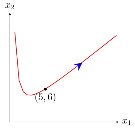
Example. Suppose a particle is moving in a planar force field and its position vector \(\overrightarrow{x}\) satisfies the IVP \[\overrightarrow{x}'=A \overrightarrow{x},\; \overrightarrow{x}(0)=[5,\;6]^T,\] where \(A=\left[\begin{array}{rr} 2&0\\4&-3\end{array} \right]\). Solve the IVP and sketch the trajectory of the particle on \(\mathbb R^2\).

Solution. The eigenvalues of \(A\) are \(2\) and \(-3\) with corresponding eigenvectors \(\left[\begin{array}{r}5\\4\end{array} \right]\) and \(\left[\begin{array}{r}0\\1\end{array} \right]\) respectively (show all the steps). So the general solution is \[\overrightarrow{x}(t)=c_1e^{2t}\left[\begin{array}{r}5\\4\end{array} \right] +c_2e^{-3t}\left[\begin{array}{r}0\\1\end{array} \right].\] \[\begin{align*} \overrightarrow{x}(0)=\left[\begin{array}{c}5\\6\end{array} \right] &\implies c_1\left[\begin{array}{r}5\\4\end{array} \right] +c_2\left[\begin{array}{r}0\\1\end{array} \right]=\left[\begin{array}{c}5\\6\end{array} \right]\\ &\implies 5c_1=5,\; 4c_1+c_2=6\\ &\implies c_1=1,\; c_2=2. \end{align*}\] So the solution is \[\overrightarrow{x}(t)=e^{2t}\left[\begin{array}{r}5\\4\end{array} \right] +2e^{-3t}\left[\begin{array}{r}0\\1\end{array} \right].\]

Geometric view: \[\overrightarrow{x}(t)=e^{2t}\left[\begin{array}{r}5\\4\end{array} \right] +2e^{-3t}\left[\begin{array}{r}0\\1\end{array} \right] =\left[\begin{array}{l}5e^{2t}\\4e^{2t}+2e^{-3t}\end{array} \right] \implies x_1=5e^{2t},\; x_2=4e^{2t}+2e^{-3t}.\] Eliminating \(t\) by using \(e^t=\sqrt{x_1/5}\), we get \(x_1^3(4x_1-5x_2)^2=1250\), the trajectory of the particle whose planar motion is described by the given IVP.

Last edited